Combining Pivot Tables, Charts, and Universal Slicers

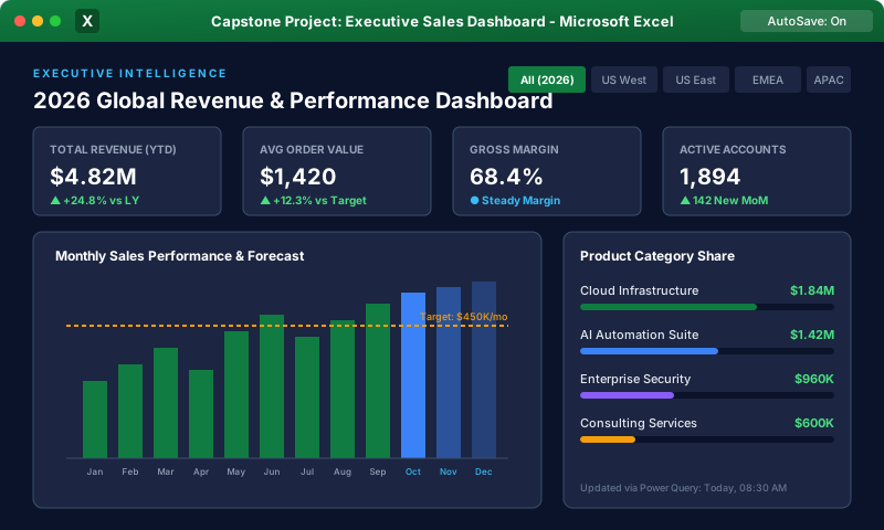
The true power of an executive dashboard emerges when individual components—KPI cards, monthly trendlines, regional distribution charts, and product rankings—are linked to Universal Slicers. With a single click on a slicer button, every visual across the dashboard recalculates and updates in synchronized harmony.

1. The Architecture of Multi-Pivot Synchronization

Click to Zoom

2. Step-by-Step Configuration: Universal Report Connections

To synchronize multiple components to a single master slicer set:

1. 1
   Build Your Specialized Pivot Tables on the 'Calc_Pivots' Tab:

• Pivot 1 (Trend): Date in Rows, Revenue & Profit in Values.
• Pivot 2 (Region): Region in Rows, Revenue in Values.
• Pivot 3 (Product): Product Name in Rows, Units & Revenue in Values.

1. 1
   Give Each Pivot Table a Descriptive Name (Best Practice!):

• Click Pivot 1 > PivotTable Analyze > rename from default 'PivotTable1' to PT_Trend.
• Rename Pivot 2 to PT_Region.
• Rename Pivot 3 to PT_Product.

1. 1
   Insert the Master Slicers:

• Click inside 'PT_Trend' > click Insert Slicer.
• Check Region, Fiscal Year, and Product Line.
• Cut (Ctrl + X) the slicers from the calculation sheet and Paste (Ctrl + V) them into the header banner of your Executive_Dashboard tab.

1. 1
   Connect All Tables via Report Connections:

• Right-click the Fiscal Year slicer > select Report Connections....
• In the dialog box, check the boxes for PT_Trend, PT_Region, and PT_Product!
• Repeat for the Region and Product Line slicers.

1. 1
   Click OK.

3. Designing Dynamic Chart Titles Linked to Slicers

Executive charts should state what is currently being filtered:

1. 1
   In cell E2 on your calculation tab, write a dynamic title formula:

1. 1
   Click the Chart Title of your Pivot Chart.
2. 2
   Click into the Formula Bar and type:

1. 1
   Press Enter.

Now, when the user clicks "West", the chart title dynamically changes to: "Monthly Revenue Performance - West"!

Multiple Choice Questions

1. Why should you assign clear custom names (like PT_SalesTrend) to Pivot Tables before configuring slicers?

A. Excel will not save unnamed Pivot Tables B. In the Report Connections dialog, descriptive names ensure you know exactly which Pivot Tables you are linking C. It encrypts the data D. It changes the table font to bold Answer: B Explanation: Descriptive Pivot Table names prevent confusion in the Report Connections checklist, ensuring filters are routed to the intended tables.

2. How do you move an inserted Slicer from the calculation staging tab to the presentation dashboard tab?

A. Retype the slicer B. Cut the slicer (Ctrl + X), navigate to the Dashboard tab, and Paste (Ctrl + V) C. Export as an image D. Slicers cannot be moved between tabs Answer: B Explanation: Slicers are floating graphic objects; cutting and pasting transfers them across sheets without severing their underlying Pivot Table links.

3. What happens if you forget to check a Pivot Table in a Slicer's Report Connections dialog?

A. Excel generates a #REF! error B. That specific Pivot Table and its linked charts will ignore the slicer, remaining static while other visuals filter C. The entire workbook locks D. The slicer disappears Answer: B Explanation: Slicers only broadcast filter context to checked Pivot Tables; unchecked tables remain unaffected by user button selections.

4. How can you make a Pivot Chart's title update dynamically to reflect the user's active slicer selection?

A. Manually retype it every time you click a button B. Link the Chart Title element to a calculation cell containing a dynamic text formula using the Formula Bar C. Use WordArt D. Set chart font to Auto Answer: B Explanation: Selecting the Chart Title element and entering a cell reference in the Formula Bar dynamically binds the title to formula output.

5. In DAX or modern Excel modeling, which function retrieves the single value currently selected by a slicer?

A. GETSLICER() B. SELECTEDVALUE() C. CURRENT() D. ACTIVE() Answer: B Explanation: SELECTEDVALUE() returns the context value when a column is filtered to a single unique item, enabling dynamic labels.