Capstone Project: Computer Vision & Monte Carlo Simulation

To solidify your mastery of NumPy, this comprehensive Capstone brings together every core concept you have learned—vectorization, multi-dimensional array slicing, broadcasting, linear algebra, universal functions, and random generators—across two complete end-to-end industry applications:

1. 1
   Computer Vision Pipeline: Constructing an image filter, color-to-grayscale luminosity transformation, and 2D spatial convolution kernel for image blurring and edge detection.
2. 2
   Quantitative Finance Engine: Vectorized Monte Carlo simulation modeling 10,000 geometric Brownian motion asset price paths to evaluate options pricing and Value-at-Risk (VaR).

Click to Zoom

Project Part 1: Computer Vision & Spatial Image Convolution

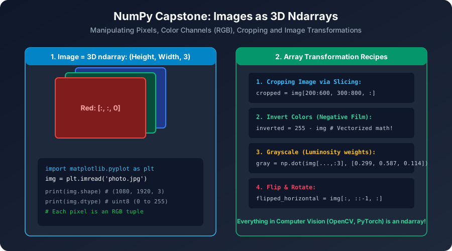
In computer vision, an image is represented as a 3D NumPy array of shape $(H, W, C)$, where $H$ is height, $W$ is width, and $C=3$ represents the Red, Green, and Blue color channels (values in range $[0, 255]$).

1. Vectorized Grayscale Conversion (ITU-R BT.601)

Human visual perception is unequally sensitive to color wavelengths. The international standard for converting RGB to grayscale weights the channels as follows:

$$Y = 0.2989 R + 0.5870 G + 0.1140 B$$

Using matrix multiplication (@), we can convert an entire image to grayscale in a single vectorized operation:

2. 2D Spatial Convolution Filter (Gaussian Blur & Edge Detection)

Image filtering (convolution) slides a small $K \times K$ kernel matrix across an image, computing the element-wise sum-product at each receptive field.

Let's implement a Gaussian Blur filter using vectorized NumPy slicing:

Project Part 2: Quantitative Finance Monte Carlo Simulation

In financial quantitative risk management, Monte Carlo simulation models future stock price uncertainty under Geometric Brownian Motion (GBM):

$$S_t = S_{t-1} \exp\left( \left(\mu - \frac{1}{2} \sigma^2\right) \Delta t + \sigma \sqrt{\Delta t} \, Z_t \right)$$

Where:

• $S_0$: Current initial stock price ($100.00).
• $\mu$: Expected annual drift rate ($8\%$ or $0.08$).
• $\sigma$: Annual volatility ($25\%$ or $0.25$).
• $\Delta t$: Time step ($1 / 252$ trading days per year).
• $Z_t \sim \mathcal{N}(0, 1)$: Standard normal random shock.

Vectorizing 10,000 Paths Across 252 Trading Days

A naive Python loop iterating over 10,000 paths and 252 days would require 2.5 million slow loop cycles. In NumPy, we generate the entire 2D matrix at once and simulate all paths simultaneously using np.cumprod():

Risk Analytics & Value-at-Risk (VaR)

With our simulated price matrix, we can extract quantitative risk metrics in milliseconds:

Output:

3. Summary of NumPy Architectural Mastery

Congratulations on completing the NumPy Complete Course! You now possess comprehensive mastery of:

• Memory layouts, contiguous C vs Fortran strides, and memory pointers.
• Sub-millisecond vectorization and universal functions (ufuncs).
• Multi-dimensional slicing, strides, views vs copies, and broadcasting mechanics.
• Production-grade linear algebra decompositions, matrix solvers, and LAPACK interfaces.
• Modern thread-safe pseudo-random generators.
• Processing gigabyte-scale datasets out-of-core with memory-mapped arrays.

You are now fully equipped to build cutting-edge data science, artificial intelligence, and scientific computing systems!

Multiple Choice Questions

1. In the grayscale conversion equation grayscale = rgb_image @ weights, why does the @ operator successfully contract the color channels?

A. It flattens the image into a 1D vector B. It computes an inner dot product between the 3 color channels of each pixel and the 3 weights, reducing shape (H, W, 3) to (H, W) C. It applies a Gaussian blur D. It normalizes pixel values between 0.0 and 1.0 Answer: B Explanation: The matrix multiplication operator @ pairs the trailing dimension of size 3 in the image with the length-3 weight vector, computing $0.2989R + 0.5870G + 0.1140B$ at every pixel.

2. In the Monte Carlo asset simulation, which NumPy function computes the compound price trajectories across time steps simultaneously?

A. np.sum() B. np.cumprod(..., axis=1) C. np.linalg.eig() D. np.gradient() Answer: B Explanation: np.cumprod(..., axis=1) computes the cumulative running product along the time axis (columns), multiplying daily return factors to evolve prices across all 10,000 paths at once.

3. What does a 95% Value-at-Risk (VaR) of $27.84 on a $100 investment indicate?

A. The average profit will be $27.84 B. In 95% of simulated market scenarios, losses will not exceed $27.84 (the loss is worse only 5% of the time) C. The stock will decrease by exactly $27.84 D. 95% of investors lose money Answer: B Explanation: Value-at-Risk (VaR) is a standard risk metric. A 95% 1-year VaR of $27.84 means that under normal market conditions, there is only a 5% probability that the portfolio loses more than $27.84 over the year.

4. Why does applying a 2D convolution kernel across an image require border padding (e.g. np.pad)?

A. To prevent integer overflow B. Because kernel windows centered on edge pixels extend beyond the original array boundaries C. To convert RGB into BGR format D. Padding is required by GPU memory alignment Answer: B Explanation: A $K imes K$ filter centered on border pixels needs neighboring pixels outside the image bounds. Padding adds border pixels (e.g. zeros or reflected values) to maintain valid convolution boundaries.

5. Why is vectorizing the Monte Carlo simulation across a 2D matrix (10000, 252) vastly superior to writing nested Python loops?

A. Nested Python loops in CPython suffer from interpreter dispatch overhead, taking seconds or minutes, while NumPy executes in milliseconds using compiled C loops and CPU vector registers B. Python loops cannot compute exponential functions C. NumPy arrays automatically predict the stock market D. Floating-point numbers cannot be stored in Python lists Answer: A Explanation: In CPython, executing millions of scalar iterations inside nested loops incurs severe dynamic typing, object allocation, and method resolution overhead. NumPy delegates the entire calculation to SIMD-optimized C loops in milliseconds.